Kristoffer Nielbo & Ryan Nichols
After the transformed data set is preprocessed with numerical representations, we can apply a text mining technique. The goal of this step is to model the data and extract a general pattern. While Natural Language Processing and Information Retrieval deliver the resources for transforming unstructured data into a numerical representation, text mining applies a range of techniques for extracting patterns as well as procedures for applying methods to the data.
For Humanities scholars, one of the primary challenges lies in identifying a specific technique that can answer the research question. One way of approaching this issue is by answering two questions. Firstly, what level of analysis are you interested in: words, words or n-gram-level relations, or documents-level relations? Secondly, how many documents does your research corpus contain: 1s, 10s, 100s or 1000s? While the first question will tell you which set of techniques to choose, the second points to restrictions on your methods. Keep in mind that most techniques require a large number of documents for reliable results, including simpler techniques like correlation estimates of word-level similarity.
In this article and in the few to follow, we will discuss various text mining techniques in an ascending order of required target documents. Techniques for word counting can be applied to only one document (we focus on word counting in this post), while techniques for modeling relations between words require more documents, and document-level modeling requires many documents.
Let’s focus on word counting. Count-based evaluation methods have a long tradition in the Humanities, as indicated by the amount of effort invested in pre-computer age concordances. In their most rudimentary form, these methods determine the number of times each word occurs for every document in the corpus and arranges them in a searchable list.
One of several weighting schemes is typically applied to the word frequencies. Relative frequency weighting is very common. This technique normalizes the frequency by the total number of words in the document or corpus. This weighting scheme can be used to estimate relative importance of a word when the documents are not the same length. Term frequency-inverse document frequency (TFIDF) weighting is another widespread weighting scheme (Manning, Raghavan & Schütze 2008) that solves the problem of all words being given equal importance.
All words, however, are not equally good at discriminating between documents. Analyses show that optimal term discrimination is obtained by words that appear a lot within a document, but do not appear so much when looking at all the documents together. ‘God’ for instance has low term discrimination in the New Testament corpus, because it occurs in every document, while ‘Mary’ has good term discrimination because it only occurs in the historical books (with the exception of Romans). The keyword ‘Mary’ can, in other words, be used to identify the historical books, while ‘God’ cannot. Weighting term frequency by the inverse document frequency removes words like ‘God’ from the New Testament, which does not help us discriminate between documents.
Computing word frequencies can be used for a range of analyses on its own, or it can supplement other advanced text mining techniques. For instance, finding the distribution of keywords in documents can be useful for exploring the presence of central characters in books (figure 1a). Also, statistics that summarize a corpus can be calculated directly from word frequencies (Jockers 2014). The Type-Token Ratio statistic (figure 1c), which measures vocabulary variation, can be used to estimate the diversity of words an author uses. But these types of statistics are negatively correlated with document length. This makes it important that the documents you look at are of similar length.
Applying a Part of Speech (POS) tagger to the research corpus makes it possible to count classes of words instead of keywords. Besides being able to count syntactic word classes, POS taggers can be used for Named Entity Recognition (NER). This can be useful when looking at historical texts. NER extracts particular entities like persons and locations from documents, making it possible to identify specific groups and estimate the relative importance of these entities in and across documents. NER should be used with caution when mining historical texts because tagging is typically developed for contemporary languages and entity identifiers can have changed over time (e.g., ‘Org’ (i.e., ‘Organization’) in figure 3b).
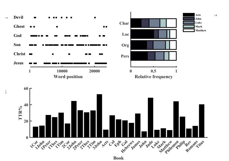
Figure 1: Word Counting (clockwise from upper left corner): a) Word position of central characters in the Gospel of Matthew. ‘Jesus’, ‘Son’ and to some extent ‘God’ are represented throughout the narrative, while ‘Christ’, ‘Devil’ and ‘(Holy) Ghost’ seem the have more specific functions in the plot. b) Name Entity Recognition for entities Person (Pers), Organization (Org), and Location (Loc). Relative to document length (Char) Acts, which account the history of several persons and their travels, has more mentions of Persons and Locations than any other book in NT. Organization here is misleading because it primarily captures Person entities due to the archaic nature of the KJV Bible. c) Type-token ratios (TTR) for each book of NT. Notice that the Gospels, which are the longest documents of NT, have the lowest TTR.
Instead of counting frequencies of words and word classes, it is possible to estimate how two or more words are associated in a research corpus (Tan, Steinbach & Kumar 2005). For example, ‘Jesus’ occurs in 26 books and ‘said’ in 14 books out of 27 books of New Testament. At mere chance level they would occur together in almost 50% of the books, while, in actuality, they occur together in 52% of the books. This does not mean that ‘Jesus’ is always the subject for ‘said.’ The association model only tells us whether or not the words occur together somewhere in each book, not their relation to each other in each instance. Document size therefore becomes extremely important for association mining, because it determines the unit of comparison. ‘Jesus’ and ‘said’ may seem to be associated differently whether we are looking at verses or books (‘said’ is actually more strongly associated with ‘Jesus’ in verse). There are many techniques for conducting association mining, but we will focus on examples of probabilistic and geometric approaches, respectively. Both approaches estimate association strength between words in a collection of documents, but differ in terms of mathematical concepts.
Probabilistic approaches often represent word relations as a co-occurrence matrix over a collection of documents (Banchs 2013). A co-occurrence matrix is a square matrix in which each word type in the corpus vocabulary is given a row and column. The New Testament has 1537 word types, so the co-occurrence matrix of the preprocessed corpus will have 1537 rows and columns, as shown in figure 2. Each entry, found across a row and down a column, tells how many documents those two words occur together. Every entry in the main diagonal will have the same word for its row and column, so it represents the number of documents a specific word occurs in.
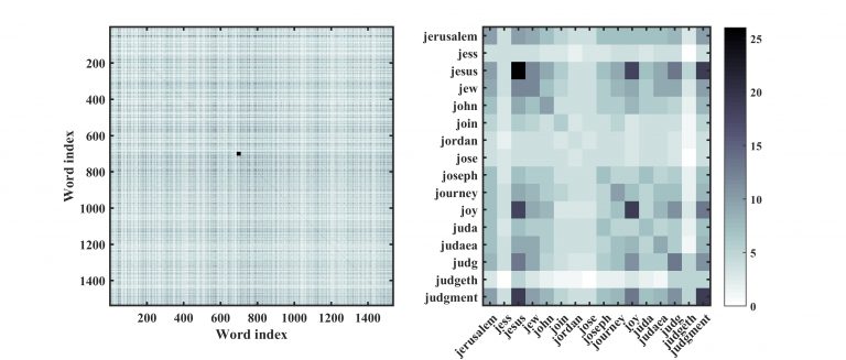
Figure 2: A co-occurrence (left to right): a) the full co-occurrence matrix of the preprocessed NT corpus. Each entry represent the number of documents wordi and wordj co-occurs in (white equals zero document co-occurrence and black 27 documents co-occurrences). b) a closer look at 16 word co-occurrences in the matrix (small square in 4a at indices 691 to 706). ‘Jesus’ is present in 26 documents (dark square on main diagonal) and co-occurs in many documents with ‘joy’ (18 documents) and ‘judgement’ (19 document).
The row and column number for ‘Jesus’ is 693 and the entry for row 693 and column 693 shows that ‘Jesus’ occurs in 26 documents (‘Jesus’ is absent in The Third Epistle of John). Entry combinations 693 (‘Jesus’) and 1099 (‘said’) show that ‘Jesus’ and ‘said’ co-occur in 14 documents. Using the co-occurrence matrix, it is possible to calculate the probabilities that words occur together (e.g., Michelbacher, Evert & Schütze 2007). The probability of encountering ‘Jesus’ in the NT books when encountering ‘said’ is 1, P(Jesus|said) = 1. The reverse, however, does not hold because ‘Jesus’ occurs in documents where ‘said’ does not, P(said|Jesus) = 0.54. The probability that ‘Jesus’ and ‘said’ co-occur is not as strong as other word associations, such as ‘Jesus’ and ‘Christ’ and ‘Jesus’ and ‘father’. Notice that this straightforward calculation of the probability of co-occurrence is done twice. Many plug-and-play corpus linguistics software platforms come stocked with clickable statistical testing, for example, the helpful, easy-to-use Sketch Engine. These tests often include ‘mutual information’ scores. While they can tell you something about the relationship between pairs of words in your corpus, mutual information (MI) scores, among others, fail to inform users about directionality of the relationship. For this reason, use of MI scores are likely to be misleading.
Some text mining techniques compare documents to see whether they contain words with a shared relation to theoretical constructs. Such constructs can vary in their level of specificity, ranging from sentiment analysis of very general subjective qualities (positive/neutral/negative) to highly detailed dictionaries of cognition, moral values, and personality (Tausczik & Pennebaker 2010; regarding Pennebaker, see our earlier posts about the Linguistic Inquiry and Word Count software tool and our accompanying instructional video.) These techniques include seeing how often words (or sequences of words) related to a construct occur in a document.
This article discussed modeling your corpus using word counting techniques. Our series of articles will continue as we focus in the next post on modeling relationships between documents.
Banchs, Rafael E. 2013. Text Mining with MATLAB. 2013 edition. Springer.
Jockers, Matthew. 2014. Text Analysis with R for Students of Literature. New York: Springer.
Manning, Christopher, Prabhakar Raghavan, and Hinrich Schütze. 2008. Introduction to Information Retrieval. 1 edition. New York: Cambridge University Press.
Michelbacher, Lukas, Stefan Evert, and Hinrich Schütze. 2007. “Asymmetric Association Measures.” Proceedings of the Recent Advances in Natural Language Processing (RANLP 2007). (Jan. 15, 2016) http://www.stefan-evert.de/PUB/MichelbacherEtc2007.pdf.
Tan, Pang-Nang, Michael Steinbach, and Vipin Kumar. 2005. Introduction to Data Mining. 1 edition. Boston: Pearson.
Tausczik, Y. R., and J. W. Pennebaker. 2010. “The Psychological Meaning of Words: LIWC and Computerized Text Analysis Methods.” Journal of Language and Social Psychology 29 (1): 24–54.